2020. 7. 31. 21:36ㆍML in Python/Python
이 게시글은 오로지 파이썬을 통한 실습만을 진행한다. 앙상블 기법중 Boosting의 개념 및 원리를 알고자하면 아래 링크를 통해학습을 진행하면 된다.
https://todayisbetterthanyesterday.tistory.com/49?category=822147
[Data Analysis 개념] Ensemble(앙상블)-3 : Boosting(Adaboost, Gradient Boosting)
1. Boosting boosting은 오분류된 데이터에 집중해 더 많은 가중치를 주는 ensemble 기법이다. 맨 처음 learner에서는 모든 데이터가 동일한 가중치를 갖는다. 하지만, 각 라운드가 종료될 때마다, 가중치
todayisbetterthanyesterday.tistory.com
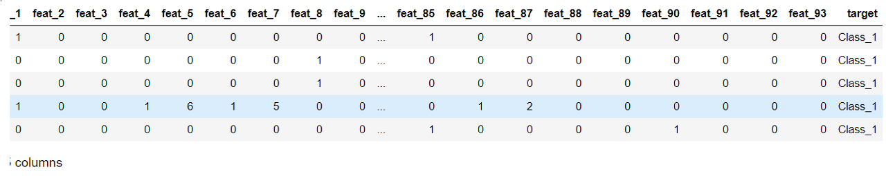
실습에 사용할 데이터는 아래의 데이터이다. kaggle에서 제공하는 데이터이며, 상세한 내용은 아래와 같다.
id: 고유 아이디
feat_1 ~ feat_93: 설명변수
target: 타겟변수 (1~9)
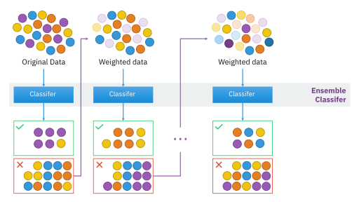
Boosting은 오분류된 데이터에 집중해 더 많은 가중치를 주는 ensemble 기법이다. 맨 처음 learner에서는 모든 데이터가 동일한 가중치를 갖는다. 하지만, 각 라운드가 종료될 때마다, 가중치와 중요도를 계산한다. 그리고 복원추출을 진행할 때 가중치의 분포를 고려한다. 가중치의 분포가 고려되며 오분류된 데이터에 가중치를 더 얻게되면서, 다음 round에서 더 많이 고려된다.
Boosting - 출처: https://commons.wikimedia.org/wiki/File:Ensemble_Boosting.svg
Boosting에는 AdaBoost, LPBoost, TotalBoost, BrownBoost, MadaBoost, LogitBoost, Gradient Boosting 등 많은 종류가 존재한다. Boosting 기법들의 차이는 오분류된 데이터를 다음 라운드에서 어떻게 반영시킬건지의 차이이다. 이 게시글에서는 가장 기본적인 boosting기법인 AdaBoost와 요즘 많이 쓰이는 Gradient Boosting에 대해서 실습을 진행할 것이다.
1. 데이터 처리
# data 처리를 위한 library

import os
import pandas as pd
import numpy as np
from sklearn.model_selection import train_test_split
# 현재경로 확인
os.getcwd()위의 코드는 파이썬 해당파일(.py / .ipynb)의 위치경로를 표기해주는 것이다. 만약 데이터가 다른 경로에 존재한다고 하였을 때, 전 경로를 확인하기 위해서 자주 사용한다.
# 데이터 불러오기
# kaggle data

data = pd.read_csv("./otto_train.csv")
data.head()
먼저 이 kaggle데이터는 target변수가 class_1~9까지 문자형식으로 되어있다. 그렇기에 이 문자형식의 target을 수치형 데이터(1~9)로 변환해줄 필요가 있다.
또한 이 kaggle데이터는 기업 및 단체가 데이터를 제공하기에 위와 같이 feature에 대한 정보를 알 수 없도록 해놓았다. 이를 통해 파이썬 실습을 진행할 것이다.
# shape확인

nCar = data.shape[0] # 데이터 개수
nVar = data.shape[1] # 변수 개수
print('nCar: %d' % nCar, 'nVar: %d' % nVar )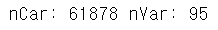
otto_train 데이터에는 61878개의 행과 95가지의 변수가 존재한다. target을 제외하면 94가지 features가 존재하는 것이다. 먼저 target의 형변환을 해주어고 무의미한 변수를 제거해야한다.
# 무의미한 변수 제거

data= data.drop(['id'],axis=1)
# 타겟 변수의 형변환
mapping_dict = {'Class_1' : 1,
'Class_2' : 2,
'Class_3' : 3,
'Class_4' : 4,
'Class_5' : 5,
'Class_6' : 6,
'Class_7' : 7,
'Class_8' : 8,
'Class_9' : 9,}
after_mapping_target = data['target'].apply(lambda x : mapping_dict[x])
after_mapping_target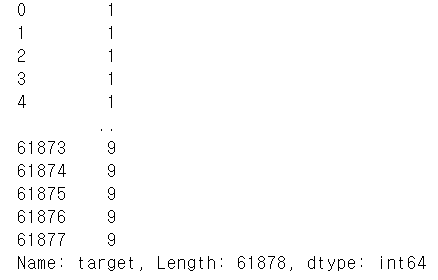
target의 형태가 "Class_1" - 1 ~ "Class_9" - 9 로 변환되었다. 이를 통해서 이제 classification을 진행할 것이다.
# features/target, train/test dataset 분리

feature_columns = list(data.columns.difference(['target']))
X = data[feature_columns]
y = after_mapping_target

train_x, test_x, train_y, test_y = train_test_split(X, y, test_size = 0.2, random_state = 42) # 학습데이터와 평가데이터의 비율을 8:2 로 분할|
print(train_x.shape, test_x.shape, train_y.shape, test_y.shape) # 데이터 개수 확인
2. AdaBoost
AdaBoost는 Boosting기법중 가장 기본적인 Boosting기법이다. Boosting의 경우는 오로지 Tree기반이 아니라 다른 모델도 함께 사용할 수 있다. AdaBoost의 parameter에 대해서 자세하게 알고싶다면 아래 sklearn 링크를 통해서 확인하는 것을 추천한다.
https://scikit-learn.org/stable/modules/generated/sklearn.ensemble.AdaBoostClassifier.html
sklearn.ensemble.AdaBoostClassifier — scikit-learn 0.23.1 documentation
scikit-learn.org
가장 기본적인 형태의 AdaBoost
# 라이브러리
from sklearn.ensemble import AdaBoostClassifier
from sklearn.tree import DecisionTreeClassifier
from sklearn.metrics import accuracy_score

# 가장 기본적인 AdaBoost
clf = AdaBoostClassifier(n_estimators=100, random_state=0)
clf.fit(train_x, train_y)
pred=clf.predict(test_x)
print(accuracy_score(test_y, pred))
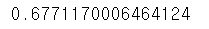
가장 기본적인 AdaBoost는 base_estimator를 아무것도 주지 않은 것이다. default값으로 설정된 model은 depth가 1인 DecisionTreeClassifier로 base_estimator = DecisionTreeClassifier(max_depth=1)로 parameter을 설정한 것과 동일한 형태이다.
이때 정확도는 대략 68%정도로 보인다.
Decision Tree 기반의 AdaBoost
# DecisionTree를 활용한 Adaboost

tree_model = DecisionTreeClassifier(max_depth=5)
clf = AdaBoostClassifier(base_estimator = tree_model, n_estimators=10, random_state=0)
clf.fit(train_x, train_y)
pred=clf.predict(test_x)
print(accuracy_score(test_y, pred))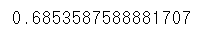
default 학습 모델 또한 DecisionTree이긴 했지만, depth설정을 해주고 이 Tree를 base_estimator에 입력해서 Tree의 역할을 하도록 만들었다. 즉 깊이를 늘린 Tree모형을 넣은 것이다. 이떄 정확도는 약간 상승하긴 했지만, 눈에 띄는 차이는 없어보인다.
추정 횟수를 증가시킨 AdaBoost
tree_model = DecisionTreeClassifier(max_depth=5)
clf = AdaBoostClassifier(base_estimator = tree_model, n_estimators=100, random_state=0)
clf.fit(train_x, train_y)
pred=clf.predict(test_x)
print(accuracy_score(test_y, pred))
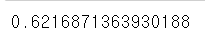
같은 DecisionTree를 가지고 추정횟수를 100회로 증가시켰다. 그랬더니 정확도는 오히려 떨어진 결과를 보인다. 이 또한 hyper parameter이기에 경험적 분석을 통해 최적의 parameter를 찾을 필요가 있다.
트리의 깊이를 증가시킨 AdaBoost
tree_model = DecisionTreeClassifier(max_depth=20)
clf = AdaBoostClassifier(base_estimator = tree_model, n_estimators=10, random_state=0)
clf.fit(train_x, train_y)
pred=clf.predict(test_x)
print(accuracy_score(test_y, pred))
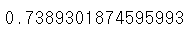
추정횟수를 줄이고 Tree의 깊이를 20으로 증가시켰더니 정확도의 상승폭이 크게 증가하였다. 이 데이터셋에서 DecisionTree를 사용할 경우 어느정도 Tree의 깊이가 필요하다는 사실을 확인할 수 있었다.
3. Gradient Boost - XGBoost
# !pip install xgboost
import xgboost as xgb
import time
start = time.time() # 시작 시간 지정
xgb_dtrain = xgb.DMatrix(data = train_x, label = train_y) # 학습 데이터를 XGBoost 모델에 맞게 변환
xgb_dtest = xgb.DMatrix(data = test_x) # 평가 데이터를 XGBoost 모델에 맞게 변환
xgb_param = {'max_depth': 10, # 트리 깊이, default = 6
         'learning_rate': 0.01, # Step Size
         'n_estimators': 100, # Number of trees, 트리 생성 개수
         'objective': 'multi:softmax', # 목적 함수    # 현재 분류 / eval_metric과 objective는 범주형/연속형 경우 나누어 작성필요
         'num_class': len(set(train_y)) + 1} # 파라미터 추가, Label must be in [0, num_class) -> num_class보다 1 커야한다.
xgb_model = xgb.train(params = xgb_param, dtrain = xgb_dtrain) # 학습 진행
xgb_model_predict = xgb_model.predict(xgb_dtest) # 평가 데이터 예측
print("Accuracy: %.2f" % (accuracy_score(test_y, xgb_model_predict) * 100), "%") # 정확도 % 계산
print("Time: %.2f" % (time.time() - start), "seconds") # 코드 실행 시간 계산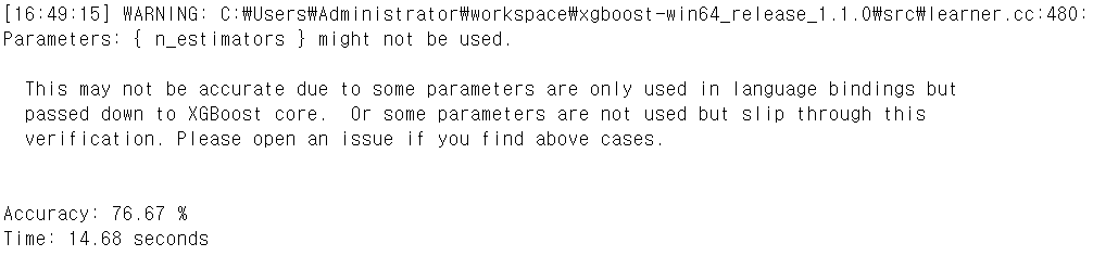
xgb_model_predict
4. Gradient Boost - LightGBM
# !pip install lightgbm
import lightgbm as lgb
start = time.time() # 시작 시간 지정
lgb_dtrain = lgb.Dataset(data = train_x, label = train_y) # 학습 데이터를 LightGBM 모델에 맞게 변환
lgb_param = {'max_depth': 10, # 트리 깊이
            'learning_rate': 0.01, # Step Size
            'n_estimators': 100, # Number of trees, 트리 생성 개수
            'objective': 'multiclass', # 목적 함수
            'num_class': len(set(train_y)) + 1} # 파라미터 추가, Label must be in [0, num_class) -> num_class보다 1 커야한다.
lgb_model = lgb.train(params = lgb_param, train_set = lgb_dtrain) # 학습 진행
lgb_model_predict = np.argmax(lgb_model.predict(test_x), axis = 1) # 평가 데이터 예측, Softmax의 결과값 중 가장 큰 값의 Label로 예측
print("Accuracy: %.2f" % (accuracy_score(test_y, lgb_model_predict) * 100), "%") # 정확도 % 계산
print("Time: %.2f" % (time.time() - start), "seconds") # 코드 실행 시간 계산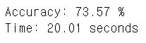
lgb_model.predict(test_x)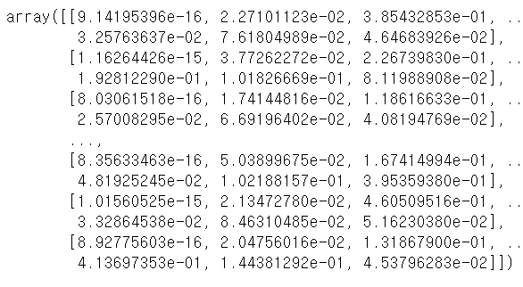
5. Gradient Boost - CatBoost
# !pip install catboost
import catboost as cb
start = time.time() # 시작 시간 지정
cb_dtrain = cb.Pool(data = train_x, label = train_y) # 학습 데이터를 Catboost 모델에 맞게 변환
cb_param = {'max_depth': 10, # 트리 깊이
            'learning_rate': 0.01, # Step Size
            'n_estimators': 100, # Number of trees, 트리 생성 개수
            'eval_metric': 'Accuracy', # 평가 척도
            'loss_function': 'MultiClass'} # 손실 함수, 목적 함수
cb_model = cb.train(pool = cb_dtrain, params = cb_param) # 학습 진행
cb_model_predict = np.argmax(cb_model.predict(test_x), axis = 1) + 1 # 평가 데이터 예측, Softmax의 결과값 중 가장 큰 값의 Label로 예측, 인덱스의 순서를 맞추기 위해 +1
print("Accuracy: %.2f" % (accuracy_score(test_y, cb_model_predict) * 100), "%") # 정확도 % 계산
print("Time: %.2f" % (time.time() - start), "seconds") # 코드 실행 시간 계산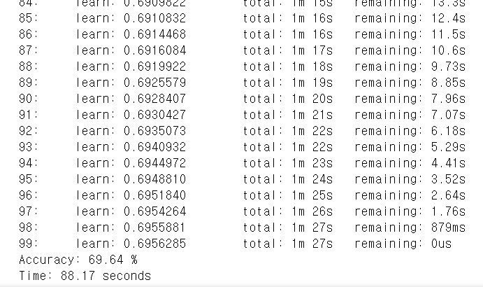
cb_model.predict(test_x)
Gradient Boosting은 기본적으로 cmd창을 통해서 install 후 함수를 갖다 쓸 수 있다. 만약 안된다면 anaconda prompt에서 conda install catboost를 통해 설치하길 바란다.
이 실습데이터에서는 XGBoost가 76%로 가장 좋은 성능과 가장 적은 시간이 걸렸다. 이는 공통 가능한 parameter일 경우 공통적으로 맞췄을 경우의 이야기이다.
하지만 일반적으로 성능은 CatBoost > LightGBM > XGBoost라고 알려져 있다. 게다가 나온 시간도 CatBoost순으로 가장 최신이기도 하다(하지만, CatBoost의 경우는 GPU를 지원하는 것으로 알려져있다). 그만큼 모델의 복잡성이 증가하고 학습시간 또한 오래 걸린다.
위의 경우들은 모두 Tree기반의 Boosting기법으로 비슷한 parameter를 갖고 활용 방법도 비슷하다. 하지만 각각의 데이터셋 설정 함수의 이름과 몇몇가지는 분명하게 다르다. 그리고 출력 결과의 shape 또한 다르다. 그렇기에 실습을 진행하고 활용을 할 때, shape의 형태와 함수이름은 잘 구분해서 쓸 필요가 있다.
'ML in Python > Python' 카테고리의 다른 글
| [Python] K-means clustering (0) | 2020.08.09 |
|---|---|
| [Python] 중요변수를 추출하기 위한 방법 - Shap Value 구현 (6) | 2020.08.03 |
| [Python] Ensemble(앙상블) - Random Forest(랜덤포레스트) (0) | 2020.07.31 |
| [Python] Ensemble(앙상블) - Bagging (0) | 2020.07.31 |
| [Python] sklearn을 활용한 인공신경망(Artificial Neural Network) 모형 실습 (0) | 2020.07.22 |