2020. 6. 24. 14:30ㆍML in Python/Python
실습에 사용될 데이터 : 개인대출 데이터
-----target
Personal Loan ( 0 or 1 의 값을 갖는 변수이다. )
-----feature
Experience 경력
Income 수입
Famliy 가족단위
CCAvg 월 카드사용량
Education 교육수준 (1: undergrad; 2, Graduate; 3; Advance )
Mortgage 가계대출
Securities account 유가증권계좌유무
CD account 양도예금증서 계좌 유무
Online 온라인계좌유무
CreidtCard 신용카드유무
※ 실습은 Ridge와 Lasso만 진행하며, ElasticNet은 개념설명만 존재합니다.
Ridge / Lasso / Elastic-Net의 개념은 아래 링크에 저장되어 있고, 이 페이지는 Python 실습만을 진행합니다.
https://todayisbetterthanyesterday.tistory.com/12
회귀계수 축소법 - Lasso, Ridge, Elastic-Net 개념
변수선택법 ※ 변수선택법으로 Forward / Backward / Stepwise 방법을 통해 유의미한 변수를 선택하여 변수의 개수를 줄이고 모델을 단순화 시키는 작업에 대해서 알아보았다. 회귀계수 축소법은 비슷��
todayisbetterthanyesterday.tistory.com
실습 (Python code)
필요 라이브러리 임포트 / 데이터 로드 및 X,Y, Train,Test Set 분리
import numpy as np
import pandas as pd
from sklearn.model_selection import train_test_split
from sklearn import metrics
from sklearn.metrics import confusion_matrix
from sklearn.metrics import accuracy_score, roc_auc_score, roc_curve
from sklearn.linear_model import Ridge, Lasso, ElasticNet
import statsmodels.api as sm
import matplotlin.pyplot as plt
import itertools
import time

ploan = pd.read_csv("./Personal Loan.csv")
ploan_processed = ploan.dropna().drop(['ID','ZIP Code'],axis=1,inplace = False)

feature_columns = list(ploan_processed.columns.difference(["Personal Loan"])
X = ploan_processed[feature_columns]
y = ploan_processed['Personal Loan'] # 대출여부 1 or 0

train_x, test_x, train_y, test_y = train_test_split(X,y,stratify = y, train_size =0.7, test_size =0.3, random_state = 42)
print(train_x.shape, test_x.shape, train_y.shape, test_y.shape)

Lasso
# Lasso 적합

ll = Lasso(alpha = 0.01 ) # alpha = Lambda
ll.fit(train_x,train_y)

alpha는 Lasso 식 상에서 lambda값이라고 하였다. 그렇기에 커지면 커질수록 회귀계수는 점점 더 0으로 수렴한다.
# 회귀계수 출력
ll.coef_
lasso와 ridge 회귀계수 축소법은 꼭 쓸모없는 변수를 줄이는 것이 아니라, 단순하게 다중공선성을 해결하고자 하는 방법이다. 그렇기에 필요한 변수의 영향력이 사라질 경우가 발생할 수도 있다.
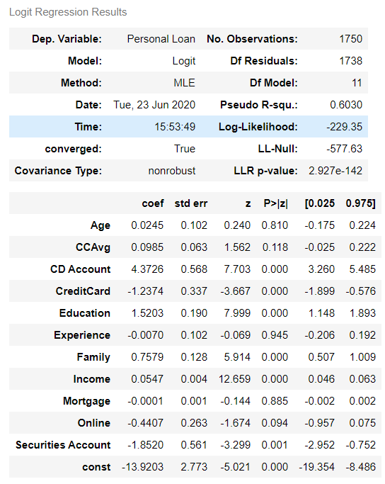
로지스틱 회귀모델의 OLS.summary()는 앞의 게시물에서 다루었다. 코드를 보고싶다면 아래 링크를 통해 접하면 된다.
https://todayisbetterthanyesterday.tistory.com/11
[Python]로지스틱회귀분석 실습
*아래 학습은 Fastcampus의 "머신러닝 A-Z까지"라는 인터넷 강의에서 실습한 내용을 복습하며 학습과정을 공유하고자 복기한 내용입니다. 실습에 사용될 데이터 : 개인대출 데이터 -----target Personal Lo
todayisbetterthanyesterday.tistory.com
※ 로지스틱 회귀모델의 계수와 비교하면 Lasso를 사용함으로써 4개의변수 (Age, CreditCard, Online, Securities Account)의 영향력이 +/-0.00000000이 된 것을 볼 수 있다. 게다가 나이와 같은 변수는 대출 가능성에 영향을 충분하게 미칠 수 있다고 생각되는 변수이나, 영향력이 Lasso에서 사라진 것을 본다면, 이는 데이터 분석을 하는 사람의 역량과 판단에 맡길 문제라고 생각된다.
##### 이 두 함수는 로지스틱 회귀모델의 게시글 코드에 존재한다.
##### Lasso와 Ridge의 예측 정확도를 측정하는데 사용할 것이다.

# 0/1 cut-off(임계값) 함수

def cut_off(y, threshold):
	Y = y.copy()
	Y[Y>threshold] = 1
	Y[Y<=threshold] = 0
	return (Y.astype(int))

# 정확도 acc 함수

def acc(cfmat):
	acc = (cfmat[0,0] + cfmat[1,1]) / np.sum(cfmat)
	return acc
## 예측, confusion matrix, acc 계산

pred_Y_lasso = ll.predict(test_x)
pred_Y_lasso = cut_off(pred_Y_lasso, 0.5)
cfmat = confusion_matrix(test_y,pred_Y_lasso)
print(acc(cfmat))
fpr,tpr, thresholds = metrix.roc_curve(test_y,pred_Y_lasso,pos_table = 1)

# print ROC curve
plt.plot(fpr,tpr)

# print AUC
auc = np.trapz(tpr, fpr)
print("AUC :",auc)
Ridge
# Lasso 적합

rr = Ridge(alpha = 0.01 ) # alpha = Lambda
rr.fit(train_x,train_y)

## ridge result
rr.coef_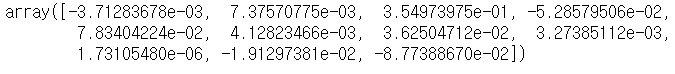
## lasso result
ll.coef_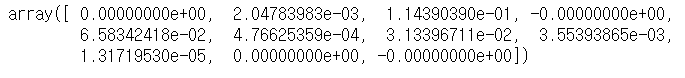
위의 Ridge와 Lasso의 결과를 보면 Lasso의 경우 회귀계수가 완전히 "0"으로 수렴한 것을 확인할 수 있지만, Ridge의 경우 0에 가까워 졌을 뿐 0은 아닌 것을 확인할 수 있다. 그렇기에 Lasso는 완전하게 특정 계수의 영향력을 무시하고 Ridge는 전반적인 모델의 회귀계수의 영향력을 줄이는(정규화작업) 것을 확인할 수 있다.
두 가지 회귀계수 축소법에 대한 차이는 게시글 맨 위의 링크를 통해 확인할 수 있다.
## ridge y 예측, confusion matrix, acc 계산
## 예측, confusion matrix, acc 계산

pred_Y_ridge = rr.predict(test_x)
pred_Y_ridge = cut_off(pred_Y_ridge,0.5)
cfmat = confusion_matrix(test_y,pred_Y_ridge)
print(acc(cfmat))
보통 정확도는 Ridge와 Elastic-Net이 좋다고 하나 약간이지만 이 데이터셋에서는 Ridge의 예측 성능이 더 좋은 것을 확인할 수 있었다. 그렇기에 회귀계수 축소법을 사용할 때는 다방면으로 확인하며 lambda값(parameter)도 여러 실험을 해보고 선택을 할 필요가 있다.
## Ridge AUC, ROC Curve
fpr, tpr, thresholds = metrics.roc_curve(test_y,pred_Y_ridge, pos_label=1)

# print ROC curve
plt.plot(fpr,tpr)

# print AUC
auc = np.trapz(tpr,fpr)
print("AUC :",auc)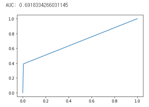
lambda 값에 따른 Lasso와 Ridge의 회귀계수 동향
# lambda값 지정
# 0.001 <= lambda <= 10

alpha = np.logspace(-3,1,5)
alpha
data = []
acc_table = []

for i, a in enumerate(alpha):
	lasso = Lasso(alpha=a).fit(train_x, train_y)
	data.append(pd.Series(np.hstack([lasso.intercept_, lasso.coef_])))
	pred_y = lasso.predict(test_x) # full model
	pred_y = cut_off(pred_y, 0.5)
	cfmat = confusion_matrix(test_y,pred_y)
	acc_table.append((acc(cfmat)))


df_lasso = pd.DataFrame(data,index = alpha).T
acc_table_lasso = pd.DataFrame(acc_table, index = alpha).T
df_lasso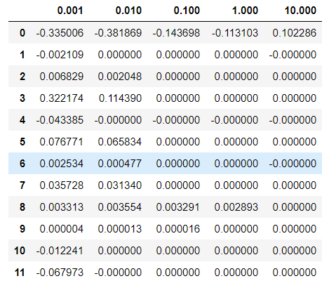
acc_table_lasso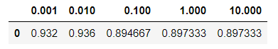
data = []
acc_table = []

for i, a in enumerate(alpha):
	ridge = ridge(alpha=a).fit(train_x, train_y)
	data.append(pd.Series(np.hstack([ridge.intercept_, ridge.coef_])))
	pred_y = ridge.predict(test_x) # full model
	pred_y = cut_off(pred_y, 0.5)
	cfmat = confusion_matrix(test_y,pred_y)
	acc_table.append((acc(cfmat)))


df_ridge = pd.DataFrame(data,index = alpha).T
acc_table_ridge = pd.DataFrame(acc_table, index = alpha).T
df_ridge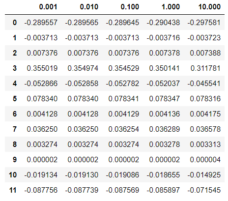
acc_table_ridge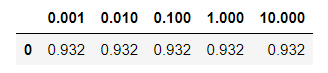
※ 위의 lambda값에 따른 두 회귀모델 축소법의 변화를 보면, Lasso는 lambda값이 커짐에 따라 대부분의 회귀계수가 0으로 수렴하는 것을 확인할 수 있는 반면, Ridge는 전반적인 수치가 정규화 되는 것을 보인다.(큰 값은 줄어들고, 작은 값은 커진다.)
이는 시각화를 통해서도 확인할 수 있다.
## 시각화
import matplotlib.pyplot as plt

ax1 = plt.subplot(121)
plt.semilogx(df_ridge.T)
plt.xticks(alpha)
plt.title("Ridge")

ax2 = plt.subplot(122)
plt.semilogx(df_lasso.T)
plt.xticks(alpha)
plt.title("Lasso")

plt.show()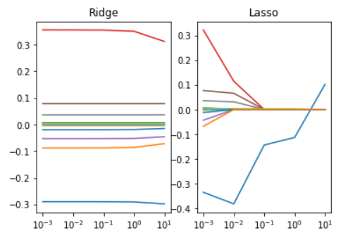
오늘은 Ridge와 Lasso의 실습코드에 대해 알아보았다. Elastic-Net은 두 모델을 합친 것으로 코드를 작성하진 않았지만, 하는 방법은 비슷하다. 다음에는 PCA(주성분분석)을 공부해 보겠다.
'ML in Python > Python' 카테고리의 다른 글
| [Python] Gaussian/Multinomial Naive Bayes Classification(가우시안/다항 나이브 베이즈 분류) 실습 (0) | 2020.07.02 |
|---|---|
| [Python] - PCA(주성분분석) 실습 (0) | 2020.06.30 |
| [Python]로지스틱회귀분석 실습 (2) | 2020.06.20 |
| [Python]변수선택법 실습(2) - 전진선택법/후진소거법/단계적선택법/MAPE 모델 성능 평가 (변수선택법 실습(1)에 전처리과정 존재) (21) | 2020.06.19 |
| [Python]변수선택법 실습(1) - 변수선택법 실습 이전단계, 불필요한 변수 제거 및 가변수 추가 ~ 다중공선성 확인작업 (변수선택법의 코드는 (2)에서) (9) | 2020.06.16 |